Title here
Summary here
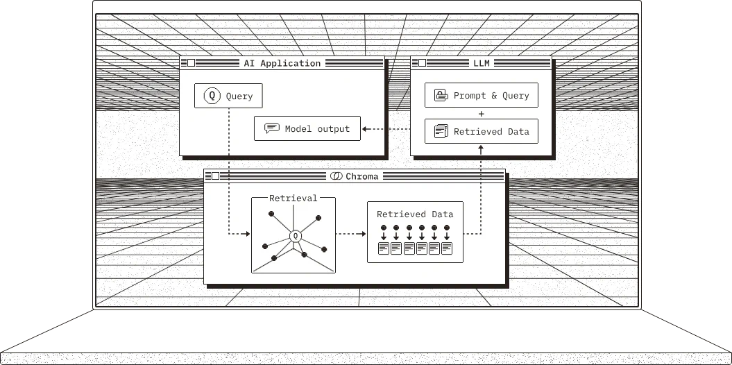
向量数据库(Vector Database)是专为处理高维向量数据设计的数据库系统,其核心技术在于将非结构化数据(如文本、图像、音频)通过深度学习模型转化为多维向量(如768维的文本嵌入向量或1024维的图像特征向量),并基于向量间的相似性实现高效检索。
| 维度 | 传统数据库 | 向量数据库 |
|---|---|---|
| 数据类型 | 结构化数据(表格、JSON) | 非结构化数据的高维向量表示 |
| 查询方式 | 精确匹配(SQL WHERE语句) | 相似度计算(余弦/欧氏距离) |
| 索引技术 | B树、哈希索引 | HNSW、LSH、KD树等近似最近邻算法 |
| 数据库 | 核心优势 | 适用场景 | 性能指标 |
|---|---|---|---|
| Milvus | 开源生态最完善,支持十亿级向量规模与混合查询 | 工业级推荐系统、基因序列分析 | 延迟<50ms @10亿向量 |
| Pinecone | 全托管云服务,分钟级部署 | 初创企业快速搭建AI应用 | 99.9% SLA,支持毫秒级响应 |
| Weaviate | 内置图神经网络,支持知识图谱与向量联合检索 | 金融风控(如反洗钱关联网络分析) | 实时数据更新,支持多模态 |
| Chroma | 与LangChain深度集成,开发者友好 | 本地化知识库(如企业文档智能问答) | 轻量级(内存占用<1GB) |
| Qdrant | 分布式架构支持PB级数据,开源商业化双轨制 | 物联网设备实时数据分析 | 吞吐量10万QPS/节点 |
下面就介绍一下比较简单的 Chroma 数据库是如何使用的:
Chroma 特点:开源、轻量级架构,与LangChain框架深度集成,支持快速搭建RAG应用。 适用场景:原型验证(如智能问答系统)、中小企业内部知识库管理。
官网地址:https://www.trychroma.com/
pip install chromadb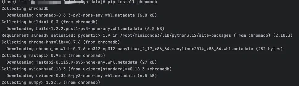
运行,其中 host 与 port 是可选的:
(base) [root@-1m466ey0ga data]# chroma run --host 127.0.0.1 --port 8000


                (((((((((    (((((####
             ((((((((((((((((((((((#########
           ((((((((((((((((((((((((###########
         ((((((((((((((((((((((((((############
        (((((((((((((((((((((((((((#############
        (((((((((((((((((((((((((((#############
         (((((((((((((((((((((((((##############
         ((((((((((((((((((((((((##############
           (((((((((((((((((((((#############
             ((((((((((((((((##############
                (((((((((    #########


Running Chroma

Saving data to: ./chroma_data
Connect to chroma at: http://127.0.0.1:8000
Getting started guide: https://docs.trychroma.com/getting-started


WARNING:  [28-02-2025 17:47:14] chroma_server_nofile is set to 65535, but this is less than current soft limit of 1000000. chroma_server_nofile will not be set.
INFO:     [28-02-2025 17:47:14] Anonymized telemetry enabled. See                     https://docs.trychroma.com/telemetry for more information.
DEBUG:    [28-02-2025 17:47:14] Starting component System
DEBUG:    [28-02-2025 17:47:14] Starting component OpenTelemetryClient
DEBUG:    [28-02-2025 17:47:14] Starting component SqliteDB
DEBUG:    [28-02-2025 17:47:14] Starting component SimpleQuotaEnforcer
DEBUG:    [28-02-2025 17:47:14] Starting component Posthog
DEBUG:    [28-02-2025 17:47:14] Starting component SimpleRateLimitEnforcer
DEBUG:    [28-02-2025 17:47:14] Starting component LocalSegmentManager
DEBUG:    [28-02-2025 17:47:14] Starting component LocalExecutor
DEBUG:    [28-02-2025 17:47:14] Starting component SegmentAPI
DEBUG:    [28-02-2025 17:47:14] Starting component SimpleAsyncRateLimitEnforcer
INFO:     [28-02-2025 17:47:14] Started server process [903657]
INFO:     [28-02-2025 17:47:14] Waiting for application startup.
INFO:     [28-02-2025 17:47:14] Application startup complete.
INFO:     [28-02-2025 17:47:14] Uvicorn running on http://127.0.0.1:8000 (Press CTRL+C to quit)
WARNING:  [28-02-2025 17:47:20] Retrying (Retry(total=1, connect=None, read=None, redirect=None, status=None)) after connection broken by 'SSLError(SSLError(1, '[SSL: WRONG_VERSION_NUMBER] wrong version number (_ssl.c:1010)'))': /batch/
看到这里,就说明运行成功了
跑起来之后我们来测试一下:
import json
import chromadb

def test_chromadb():
    # 初始化
    client = chromadb.HttpClient()
    # 创建之前先删除 collection,并且二次运行代码报错
    client.delete_collection("sample_collection")
    # 创建 collection
    collection = client.create_collection("sample_collection")
    # Add docs to the collection. Can also update and delete. Row-based API coming soon!
    collection.add(
        documents=["This is document1", "This is document2"],  # we embed for you, or bring your own
        metadatas=[{"source": "notion"}, {"source": "google-docs"}],  # filter on arbitrary metadata!
        ids=["doc1", "doc2"],  # must be unique for each doc
    )
    results = collection.query(
        query_texts=["This is a query document"],
        n_results=2,
        # where={"metadata_field": "is_equal_to_this"}, # optional filter
        # where_document={"$contains":"search_string"}  # optional filter
    )
    print(json.dumps(results))


# Press the green button in the gutter to run the script.
if __name__ == '__main__':
    test_chromadb()
这是输出结果, 可以看到两个关联的结果都被查出来了:
{
    "ids": [
        [
            "doc1",
            "doc2"
        ]
    ],
    "distances": [
        [
            0.9026352763806998,
            1.0358158255050436
        ]
    ],
    "embeddings": null,
    "metadatas": [
        [
            {
                "source": "notion"
            },
            {
                "source": "google-docs"
            }
        ]
    ],
    "documents": [
        [
            "This is document1",
            "This is document2"
        ]
    ],
    "uris": null,
    "data": null,
    "included": [
        "distances",
        "documents",
        "metadatas"
    ]
}
其中 distances 表示相关性的距离,距离越大,就标明相关性越低,我们可以举例一个反例:
def test_chromadb():
    client = chromadb.HttpClient()
    client.delete_collection("sample_collection")
    collection = client.create_collection("sample_collection")
    collection.add(
    # 增加一条新的文档 video
        documents=["This is document1", "This is document2", "This is a video"],
        metadatas=[{"source": "notion"}, {"source": "google-docs"}, {"source": "test-dir"}],
        ids=["doc1", "doc2", 'videoDir'],
    )
    results = collection.query(
        query_texts=["This is a query document"],
        # 查询结果,最多返回 10 条
        n_results=10,
    )
    print(json.dumps(results))
结果如下:
{
    "ids": [
        [
            "doc1",
            "doc2",
            "videoDir"
        ]
    ],
    "distances": [
        [
            0.9026352763806998,
            1.0358158255050436,
            1.6698303861664785
        ]
    ],
    "embeddings": null,
    "metadatas": [
        [
            {
                "source": "notion"
            },
            {
                "source": "google-docs"
            },
            {
                "source": "test-dir"
            }
        ]
    ],
    "documents": [
        [
            "This is document1",
            "This is document2",
            "This is a video"
        ]
    ],
    "uris": null,
    "data": null,
    "included": [
        "distances",
        "documents",
        "metadatas"
    ]
}
我们可以看到,第三条的结果是的距离是 1.6,可以说相关性是非常小了,如果把 n_results=10, 只返回两条的话,那数据库
就只会返回前面两个结果,第三个结果不会返回。
distances 是一个浮点数列表,表示查询向量与每个返回结果向量之间的距离。
ChromaDB 默认就是使用欧氏距离来判断查询向量与结果向量之间的距离,距离越小,相似度越高。
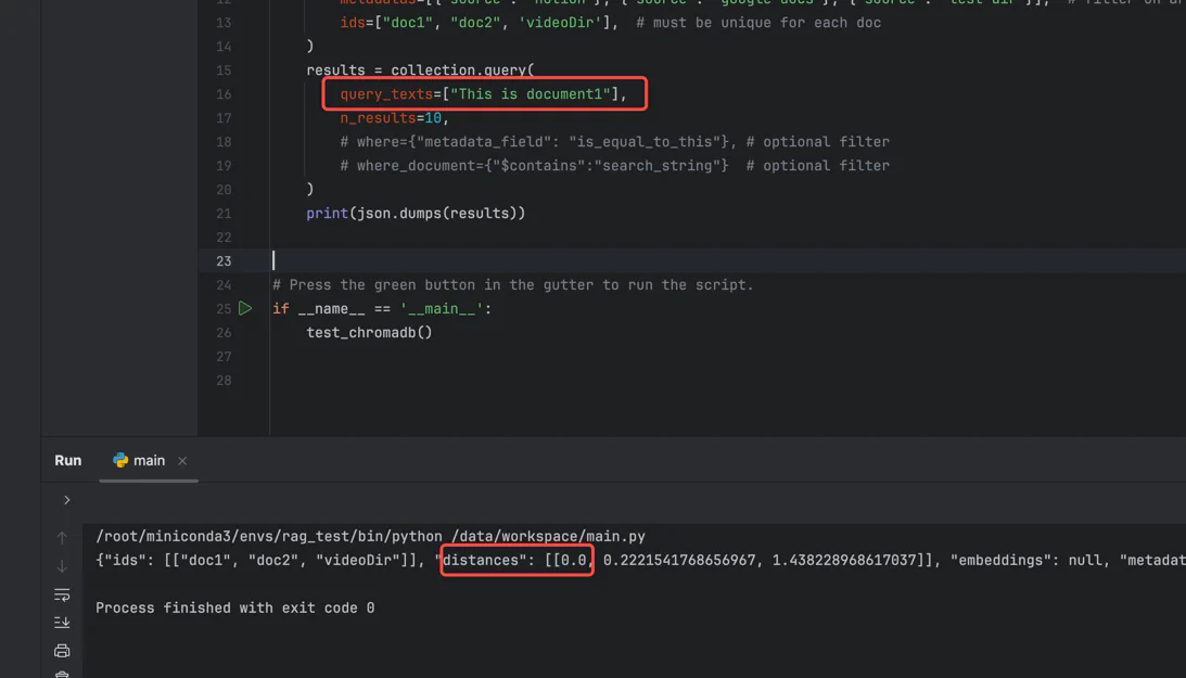
我们稍微修改一下差距的句子,改成跟第一条一样的:This is document1 ,就会发现 distances 返回的是 0, 说明这两个文本是一样的:
当然,也可以使用余弦相似度(cosine similarity) 来计算:
def test_chromadb():
    # Use a breakpoint in the code line below to debug your script.
    client = chromadb.HttpClient()
    client.delete_collection("sample_collection")
    collection = client.create_collection("sample_collection", metadata={
        "hnsw:space": "cosine", # 改成使用余弦相似度
    })
    # Add docs to the collection. Can also update and delete. Row-based API coming soon!
    collection.add(
        documents=["This is document1", "This is document2", "This is a video"],  # we embed for you, or bring your own
        metadatas=[{"source": "notion"}, {"source": "google-docs"}, {"source": "test-dir"}],
        # filter on arbitrary metadata!
        ids=["doc1", "doc2", 'videoDir'],  # must be unique for each doc
    )
    results = collection.query(
        query_texts=["This is a query document"],
        n_results=10,
        # where={"metadata_field": "is_equal_to_this"}, # optional filter
        # where_document={"$contains":"search_string"}  # optional filter
    )
    print(json.dumps(results))
结果:
{
    "ids": [
        [
            "doc1",
            "doc2",
            "videoDir"
        ]
    ],
    "distances": [
        [
            0.45131760715362124,
            0.5179078862603612,
            0.8349151851116271
        ]
    ],
    "embeddings": null,
    "metadatas": [
        [
            {
                "source": "notion"
            },
            {
                "source": "google-docs"
            },
            {
                "source": "test-dir"
            }
        ]
    ],
    "documents": [
        [
            "This is document1",
            "This is document2",
            "This is a video"
        ]
    ],
    "uris": null,
    "data": null,
    "included": [
        "distances",
        "documents",
        "metadatas"
    ]
}
我们可以看到使用余弦相似度的话,也可以判断,数值不一样而已。
欧氏距离和余弦相似度各有优缺点,选择哪种方式取决于数据特性和应用场景。
详细可以看这里的文档:
https://docs.trychroma.com/docs/collections/configure#configuring-chroma-collections
#
学习LLM & 讨论AIGC #

每天大模型、LLM、AIGC 技术咨询